of parental alleles coming together in various genotype combinations.
[expectation: the anticipated value of a variable
Genetic variation in populationscan be
described by genotype and allele frequencies.
(not "gene" frequencies)
Consider a diploid autosomal locus
with two alleles and no dominance
(=>
semi-dominance:
AA
, Aa , aa phenotypes are distinguishable)
# AA = x # Aa = y # aa = z x + y + z = N (sample size)
f(AA) = x / N f(Aa) = y / N f(aa) = z / N
f(A) = (2x + y) / 2N f(a) = (2z + y) / 2N
or f(A) = f(AA) + 1/2 f(Aa) f(a) = f(aa) + 1/2 f(Aa)
let p = f(A), q = f(a) p & q are allele frequencies
Properties of p & q
p + q = 1 p = 1 - q q = 1 - p
(p + q)2 = p2 + 2pq + q2 = 1
(1 - q)2 + 2(1 - q)(q) + q2 = 1 [Homework: show this algebraically]
p & q are interchangeable wrt [read, "with respect to"] A & a;
q is usually used for the
rarer, recessive, or deleterious (disadvantageous) allele;
BUT 'common' &
'rare'
are statistical properties
'dominant' & 'recessive' are genotypic properties
'advantageous' & 'deleterious' are phenotypic
properties
*** combination of these properties is possible
***
What happens to p & q in one generation of random mating?
Consider a population of
monoecious organisms
reproduction by random union of
gametes
("tide pool" model)...
(1)
Determine
the expectations
of parental alleles coming together in various genotype combinations.
[expectation: the anticipated value
of a variable ![]() probability]
probability]
The probability
/ binomial
expansion
/ Punnet Square
methods
all show that expectation of f(AA) = p2
expectation of f(Aa) = 2pq
expectation of f(aa) = q2
(2) Re-describe allele frequencies among offspring (A' & a').
f(A')
= f(AA) + 1/2 f(Aa)
= p2 + (1/2)(2pq) = p2 + pq =
(p)(p+q)
= p' = p
f(a')
= f(aa) + 1/2 f(Aa)
= q2 + (1/2)(2pq) = q2 + pq =
(q)(p+q)
= q' = q
p2 : 2pq : q2 are Hardy-Weinberg proportions (cf. Mendelian ratios 1 : 2 : 1 )
[avoid the phrase "Hardy-Weinberg equilibrium":
H-W proportions occur under
non-equilibrium conditions].
The Hardy-Weinberg Theorem holds under "more realistic" conditions:
(1) multiple alleles / locus
p + q + r = 1
(p + q + r)2 = p2 + 2pq + q2 + 2qr + r2
+ 2pr = 1
The proportion of heterozygotes
(H = 'heterozygosity')
is a measure of genetic variation at a locus.
Hobs = f(Aa) = observed
heterozygosity
Hexp = 2pq = expected
heterozygosity (for two alleles)
He = 2pq + 2pr + 2qr = 1 - (p2 + q2 + r2) for three alleles
n
He = 1 - ![]() (qi)2
for n alleles
(qi)2
for n alleles
i=1
where qi = freq. of ith allele of n alleles at
a locus
Ex.: if q1 = 0.5, q2 = 0.3, & q3
= 0.2
then He = 1 - (0.52 + 0.32 +
0.22)
= 0.62
Ex.:
PopGen at ABO locus
(2) sex-linked loci
iff [read: "if and only if"]
allele frequencies in males and females are identical
If frequencies are initially unequal, they converge
over several generations.
(3) dioecious organisms
(like humans)
sexes are separate
H-W is produced by random mating of individuals (random
union
of genotypes).
expand (p2 'AA' + 2pq 'AB' + q2 'BB')2
:
nine possible 'matings' among genotypes
(See derivation)
[Also holds if no selfing (self-fertilization) is possible]
Genotype proportions in natural
populations
can be tested for H-W conditions
Ho
(null
hypothesis): no outside factors are acting.
Among North American whites:
|
|
|
|
|
|
|
|
|
|
f(M) = [(2)(1787) + 3039] / (2)(6129)= 0.539
f(N) = [(2)(1303) + 3039] / (2)(6129)= 0.461 = 1.0 - 0.539
Chi-square
(![]() 2) test:
2) test:
|
|
|
|
|
|
|
|
|
|
|
|
|
|
|
|
|
|
|
|
|
|
|
|
|
|
|
|
|
|
|
|
note:
there is only one degree of
freedom,
because there are only two alleles
|
|
|
|
|
|
|
|
|
|
|
|
|
|
|
|
|
|
|
|
|
|
|
|
|
|
|
|
|
|
|
|
Chi-square test on combined data:
|
|
|
|
|
|
|
|
|
|
|
|
|
|
|
|
|
|
|
|
|
|
|
|
|
|
|
A mixture
of
populations, each of which shows Hardy-Weinberg proportions,
will
not show expected Hardy-Weinberg proportions
if the allele frequencies are different in the separate
populations.
Wahlund Effect: an artificial
mixture
of populations
(or a structured metapopulation)
will have a
deficiency of heterozygotes
The Hardy-Weinberg conditions are the
'null
hypothesis':
What are
the consequences of other genetic / evolutionary phenomena?
How do they interact?
Five major factors:
1. Natural
selection
Change of allele frequencies (![]() q)
[read as 'delta q']
q)
[read as 'delta q']
occurs due to differential effects of alleles on 'fitness'
Consequences depend on dominance of fitness
Natural Selection is the principle concern of "microevolutionary" theory
2. Mutation
A and A' are inter-converted at some rate µ
.
If µ(A![]() A')
A') ![]() µ'(A
µ'(A![]() A'),
net change
will occur in one direction.
A'),
net change
will occur in one direction.
3. Gene
flow
Net movement of alleles between populations occurs at some rate m
.
(Im)migration
introduces new alleles, changes frequency of existing alleles.
4. Population
structure
Inbreeding: preferential mating of
relatives at some rate F (see Homework).
Non-random reproduction: variable
sex
ratio, offspring number, population ize
5. Statistical
sampling error
Chance fluctuations occur in finite populations, especially
those
with small size N.
Genetic drift: random change of
allele
frequencies
over time & among populations (see Homework)
The Mathematical Theory of Natural Selection
"Natural
Selection" is the name given to an evolutionary process
in which
"adaptation" occurs in such a way
that "fitness"
increases.
Under certain conditions, this results in descent with modification.
If:
variation
exists for some trait, and
a fitness difference is correlated
with that trait, and
the trait is to some degree heritable
(determined by genetics),
Then:
the trait distribution will change
over the life history of organisms in a single generation,
and
between generations.
The
process
of change in the population is called "adaptation"
That's
all.
Evolution
&
Natural Selection can be modeled genetically.
variation = variable p & q
fitness = differential phenotypes of
corresponding genotypes
heritability = Mendelian principles
Natural Selection results in change
of allele frequency (![]() q)
[read as "delta q"]
q)
[read as "delta q"]
in consequence of
differences
in the relative
fitness (W)
of the phenotypes to
which the alleles contribute.
Fitness is a
phenotype
of individual organisms.
Fitness is determined genetically (at least in part).
Fitness is related to success at survival AND reproduction.
Fitness can be measured & quantified (see below).
i.e., the relative fitness of genotypes can be assigned
numerical
values.
The consequences of natural selection
depend
on the dominance of fitness:
e.g., whether the "fit" phenotype is due to a dominant or
recessive
allele.
Then, allele frequency change is predicted by the General Selection Equation:
![]() q
= [pq] [(q)(W2 - W1) + (p)(W1 - W0)]
/
q
= [pq] [(q)(W2 - W1) + (p)(W1 - W0)]
/![]()
where W0,
W1,
& W2
are the fitness phenotypes
of the AA, AB, & BB genotypes,
respectively
[see derivation]
genotype:
AA AB BB
phenotype:
W0
= W1 ![]() W2 (AA and AB have
identical
phenotypes)
W2 (AA and AB have
identical
phenotypes)
Then the
GSE
simplifies to ![]() q
= pq2(W2 - W1)
(since W1 - W0 = 0)
q
= pq2(W2 - W1)
(since W1 - W0 = 0)
If 'B' phenotype is more fit than 'A' phenotype,
W2 > W1 & ![]() q
> 0 so q increases.
q
> 0 so q increases.
If 'B' phenotype is less fit than 'A' phenotype,
W2 < W1 & ![]() q
< 0 so q decreases.
q
< 0 so q decreases.
then ![]() q
q ![]() (W2 - W1)
: the greater the difference in fitness,
(W2 - W1)
: the greater the difference in fitness,
the greater the intensity of selection
and the more rapid the change
A numerical
example
of Selection:
Tay-Sachs Disease is caused by an allele
that is rare (q![]() 0.001)
0.001)
recessive (W0 = W1 = 1)
lethal (W2
= 0)
Then ![]() q
= pq2(W2 - W1) = -pq2
q
= pq2(W2 - W1) = -pq2 ![]() -q2
(since p
-q2
(since p ![]() 1)
1)
That is, Natural Selection results in a decrease in the
frequency
of
the Tay-Sachs allele of about one part in a million (0.0012)
per generation
s = 1 - W
The selection coefficient (s)
is the difference in fitness
of the phenotype relative to some 'standard' phenotype
that has a fitness W = 1
[The math is simpler because only one variable is used for fitness.]
(1) Complete dominance
genotype:
AA AB BB
phenotype:
W0 = W1 ![]() W2 (AA and AB have
identical
phenotypes)
W2 (AA and AB have
identical
phenotypes)
or 1
=
1 ![]() 1
- s
1
- s
if 0 < s < 1 : 'B' is deleterious(at
a selective disadvantage)
if s < 0 : 'B' is advantageous
then ![]() q
= -spq2 / (1 - sq2)
[see derivation]
q
= -spq2 / (1 - sq2)
[see derivation]
(2) Incomplete dominance
genotype:
AA AB
BB
phenotype:
W0 ![]() W1
W1 ![]() W2 (all phenotypes different)
W2 (all phenotypes different)
or 1
- s1 ![]() 1
1 ![]() 1
- s2
1
- s2
if 0
<
s1
& s2 < 1 : overdominance
of
fitness (heterozygote advantage)
The
population
has optimal fitness when
both alleles are retained:
q will reach an equilibrium
where ![]() q = 0
q = 0
0 < ![]() <
1
(read as, "q hat")
<
1
(read as, "q hat")
then ![]() =
(s1) / (s1 + s2)
[see derivation]
=
(s1) / (s1 + s2)
[see derivation]
Direction
of allele frequency change is due to fitness
difference
of alleles
(whether the effect of the allele on phenotype is deleterious or
advantageous).
Ultimate
consequences depend on the dominance of
fitness
(whether the allele is dominant, semi-dominant, or recessive).
Rate
of change is an interplay of both of these factors (see Lab
#1)
AA
AB BB Consequence
of natural selection [ let ![]() q
= change in f(B) ]
q
= change in f(B) ]
W0
= W1 = W2 No
selection (neither allele has a
selective
advantage):
then ![]() q
= 0, H-W proportions remain constant
q
= 0, H-W proportions remain constant
W0
= W1 > W2 deleterious
recessive (advantageous dominant):
then ![]() q
< 0, q
q
< 0, q ![]() 0.00 (loss): how fast? [Does
it get there?]
0.00 (loss): how fast? [Does
it get there?]
W0
= W1 < W2 advantageous
recessive (deleterious dominant):
then ![]() q
> 0, q
q
> 0, q ![]() 1.00 (fixation): how fast?
1.00 (fixation): how fast?
W0
< W1 > W2 overdominance
[special case of semi-dominance]:
heterozygote superiority
q ![]()
![]() , where
, where ![]() q = 0
q = 0
Short-term measures: "Life Table" parameters
rate of instantaneous increase (r) of a phenotype
recall logistic
equation:
dN / dt = rN = rN (K - N)
/ K
where K = carrying capacity
net reproductive rate: exp(r)
= er
r is "compound interest" on N
replacement rate (RO):
lifetime reproductive output
~ er(at low density)
components of fitness:
traits
that contribute to survival
&
reproduction
Ex.: survivorship (expected survival time)
fecundity (# offspring at
age x)
Adaptation is
the phenotypic consequence for populations of natural selection on
individuals
[cf.
adjust / acclimate]
Phenotypic
traits that change as a result of selection
are sometimes referred to as "adaptations"
or "adaptive characters"
Life table analysis: survivorship and fecundity vary with age
lx
= prob. of survival from birth to
age
x
(cumulative)
survivorship = probability of
survival
to age x+1 from age x
mx
= fecundity (# offspring) at age x
L
then ![]() (lx)(mx) exp(-rx) = 1
(in a stable population,
(lx)(mx) exp(-rx) = 1
(in a stable population,
x=1
where L = life expectancy)
L
Ro=![]() (lx)(mx)
(lx)(mx) ![]() replacement rate
replacement rate ![]() erat
low density
erat
low density
x=1
This
equation
is a discrete solution to the continuous logistic
equation
Consider a population with two
demographic
phenotypes:
These
phenotypes
correspond to two reproductive 'strategies
iteroparous
strategy:
offspring produced over several seasons
semelparous
strategy:
offspring produced all in one season
A survivorship
and fecundity schedule will compare their life histories
life table parameters can be measured experimentally
Under 'typical'
environmental conditions, survivorship is 50% / year:
both strategies produce 2 young / female / lifetime
=> both phenotypes are equally 'fit' [and N is
stable]
In 'good
times', survivorship increases to 75% / year:
iteroparous strategy produces 4 young / female / lifetime
semelparous strategy produces 3 young / female / lifetime
=> iteroparous phenotype is 'more fit' [and N is
increasing]
In 'bad
times', survivorship decreases to 25% / year:
iteroparous
Ro = 0.72, semelparous Ro
= 1.00
=> semelparous phenotype is 'more fit' [and N is
decreasing]
=> Population phenotypes will adapt to changing conditions
In a
favourable
environment, K increases:
e.g.,
productivity of meadow increases
iteroparity more advantageous, population density increases
In an
unfavourable
environment, r increases:
e.g.,
severity of winter highly variable
semelparity more advantageous, early reproduction favoured
K-strategy:
maintain population size N close to K
long-lived,
reproduce late, smaller # offspring, lots of parental care
E.g.,
many bird species, primates (including Homo)
r-strategy:
maximize growth potential
r
short-lived,
reproduce early, larger # offspring, little parental care
E.g.,
most invertebrates, some rodents
We can extend single-locus ![]() multilocus
multilocus ![]() quantitative models
quantitative models
p2:2pq:q2
W0,W1,W2
Mendel's Laws & H-W Theorem
![]()
![]()
![]()
normal
distribution fitness
function
heritability
Variation can be quantified (see a Primer of Statistics for review)
mean ![]() standard deviation:
standard deviation: ![]()
![]()
![]()
variance: ![]() 2
2
coefficient
of variation (CV)
= (![]() /
/![]() )
x 100
)
x 100
CV
removes
size effect when comparing variance:
Ex.: Suppose X = leg
length
Y
= eye width
X = 100 ![]() 1.0
versus
Y = 1.0
1.0
versus
Y = 1.0 ![]() 0.1
0.1
CV of X = 1% CV
of
Y = 10%
Y is more variable, though ![]() X
is larger
X
is larger
Quantitative
variation follows "normal distribution"
(bell-curve) iff
Multiple loci are involved
Each locus has about the same effect
Each locus acts independently
[interaction variance (see below) is minimal]
Variation has two sources: genetic
(![]() G2)
&
environmental
(
G2)
&
environmental
(![]() E2)
variance
E2)
variance
phenotypic variance ![]()
![]() P2
=
P2
= ![]() G2
+
G2
+ ![]() E2
+
E2
+ ![]() GxE2
GxE2
additive variance ![]()
![]() A2
=
A2
= ![]() G2
+
G2
+ ![]() E2
E2 ![]()
heritability ![]() h2 =
h2 = ![]() G2/
G2/![]() A2
=
A2
= ![]() G2
/ (
G2
/ (![]() G2
+
G2
+ ![]() E2)
E2)
"heritability in the narrow sense": ignores ![]() GxE2
GxE2 ![]() interaction variance:
interaction variance:
Identical genotypes produce different phenotypes in
different
environments.
Ex.: same breed of cows produces different milk yield on
different
feed
The Norm of
Reaction describes the relationship between genetics and environement
Artificial
breeding
indicates that
organismal variation is highly heritable
ex.:
Darwin's
pigeon breeding experiments
Artificial
selection
on agricultural species
Commercially useful traits can be improved by selective breeding
IQ
scores in Homo: h2![]() 0.7
0.7
[But: IQ scores improve with education: ![]() GxE2
is large]
GxE2
is large]
Offsrping
/ Midparent correlation
For many traits in many organisms:
CV = 5 ~ 10 %
h2 = 0.5 ~
0.9
Fitness
function
expresses relationship
between
genotype & fitness
Function is a continuous
variable, rather than discrete values for W0,
W1,
& W2
=> Most traits vary & are
heritable.
Many traits
do
respond to 'artificial' selection.
Many traits
should
respond to 'natural' selection.
=> To demonstrate & measure
Natural
Selection,
we must
show experimentally that heritable
variation has consequences for fitness
<=
Quantitative
trait distribution can be described as a bell curve
with a particular mean & variance:
What happens to this distribution under Selection?
(1) Directional Selection
Fitness
function has constant slope:
Trait mean
shifted towards favored phenotype
trait variance unaffected
In
single-locus
models, the limit of selection is
Elimination
of variation by fixation of favored allele
In quantitative
models,
rate is limited by
substitutional
genetic load:
"cost" of replacing non-favored allele (![]() "intensity" of selection)
"intensity" of selection)
"Soft"
selection
Mortality is density-dependent
In 'real' stable populations: N(after)![]() N(before)
N(before)
Survivorship is proportional to fitness up to K: more
realistic
Selection will affect recruitment to next generation
Ex.: If the first-born dies of malaria, s/he will be replaced.
More births occur such that N is continually "topped up".
Birth of succeeding offspring will maintain N near K
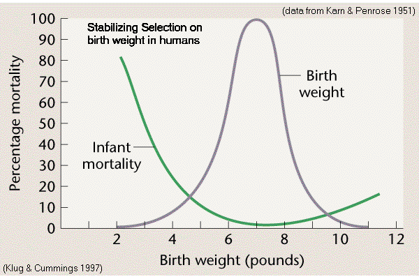
(2) Stabilizing
Selection (AKA truncation selection)
Fitness
function has a "peak"
Trait
variance reduced around (existing) optimal phenotype,
trait mean unaffected
Limits:
elimination of variant alleles
or, 'weeding out' of
disadvantageous variants
homozygosity at multiple loci:
difficult iff variance due to recessive alleles
inbreeding depression: loss of
'health'
in inbred lines
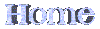
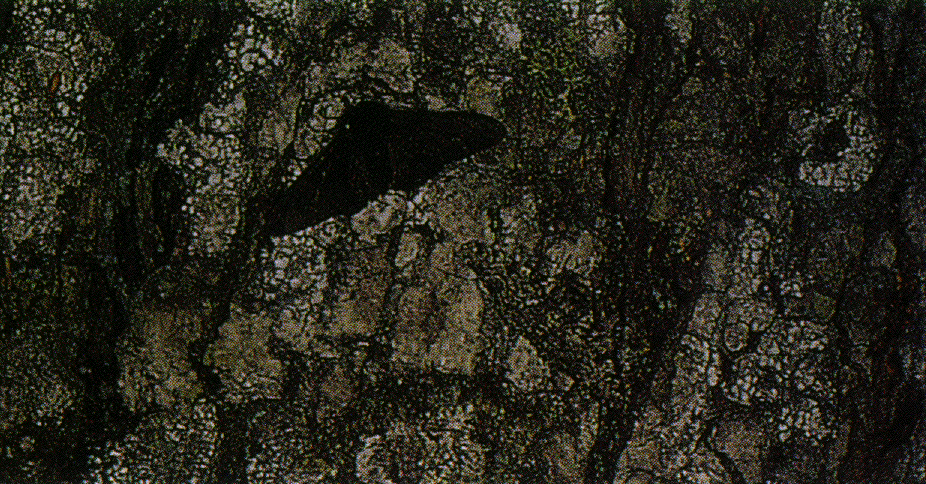
Examples:
Elimination of non-cryptic pepper moths (Biston)
melanistic variants are eliminated rapidly
in light-colored environments
peppered variants are reduced slowly
in dark-colored environments
Birthweight
in Homo (Karn & Penrose 1951)
Modal birthweight is optimum for survival
(3) Diversifying
Selection (two kinds)
There
is a lot of variation: does selection explain it?
(A) Balancing
Selection:
Fitness
function has more than one peak (multi-modal)
Overdominance:
heterozygotes
have superior fitness at a locus
because different alleles are favoured in different environments
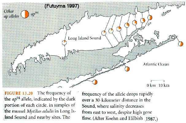
Examples:
sickle-cell
hemoglobin in Homo ('Contradictory' selection)
Leucine Aminopeptidase (LAP) & salinity
tolerance in Mytilus mussels
heterodimers:
multimeric enzymes with polypeptides from different alleles
often show wider substrate specificity, kinetic properties (Vmax
& KM)
myoglobin in
diving mammals
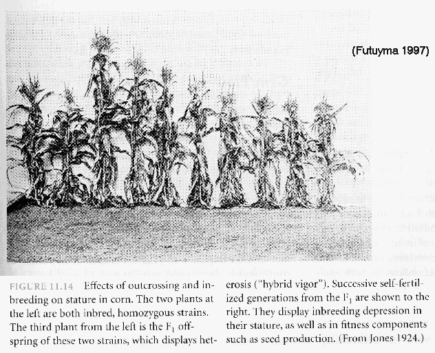
Heterosis:
heterozygosity at multiple loci improves general fitness
Hybrid
vigour: crossbreeding
of inbred lines
improves fitness in F1
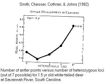
Marginal
epistasis: high 'Hobs' is 'good for you'
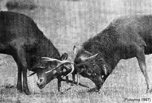
Ex.:
correlation between phenotype & genotype: antler
points in Odocoileus deer
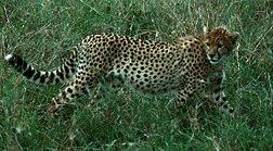
Ex.:
fluctuating
asymmetry:
Acionyx
cheetahs
are lopsided
Maintaining polymorphic phenotypic variation by selection
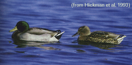
Sexual
Selection (Darwin 1871):
'exaggerated' phenotypes are disadvantageous somatically
but are favoured in competition for mates
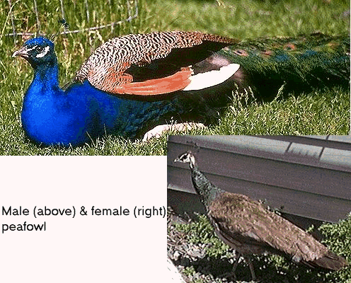
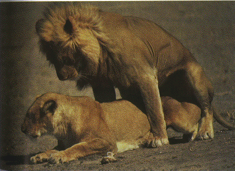
secondary sex characteristics:
Sexual dimorphism in mallards,
peafowl,
& lions
Antlers
in Cervidae are used in male-male
combat
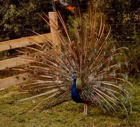
Tail
displays in peacocks attract mates
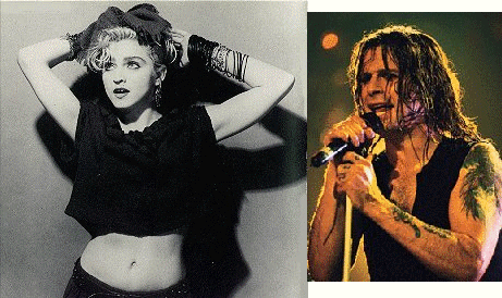
'Runaway
sexual selection': the Madonna
/ Ozzy Osborne Effect
Females choose males on basis of some distinctive trait
Offspring have exaggerated trait (males) & preference
for
trait (females)
=> selection reinforces trait & preference for trait
simultaneously
New phenotype spreads
rapidly in population
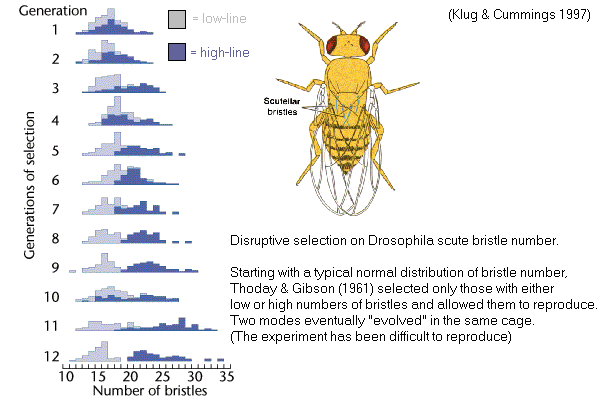
(B) Disruptive
selection
Fitness
function is a valley
Trait variance increases (like balancing), BUT polymorphism is
unstable
[Try NatSel with: q = 0.5, N = 9999, W0 = 1.0, W1 = 0.7, W2 = 1.0]
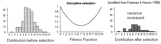
Polymorphism
can usually be maintained only temporarily:
One of the phenotypes will outcompete the other
unless
different phenotypes choose different niches (Ludwig Effect)
[and then this becomes Balancing Selection]
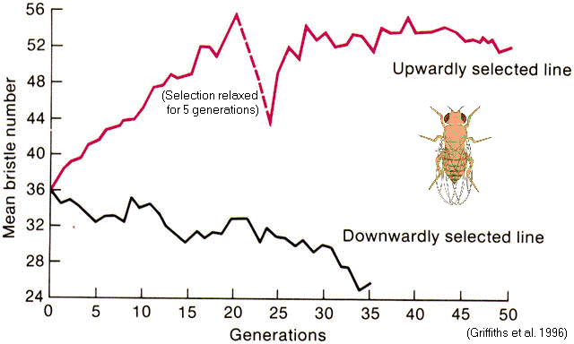
Scutellar
bristles in Drosophila (Thoday & Gibson 1962)
Selection for 'high
#' versus
'low #' lines
=> 'pseudo-populations'
with
reduced interfertility
Might disruptive selection contribute to speciation?
Natural selection is ordinarily defined
as
differential survival
& reproduction of individuals:
Can
selection
operate on other biological units?
Can such
selection 'oppose' individual selection?
Genic
(Gametic)
Selection
![]() Differential survival & 'reproduction' of alleles
Differential survival & 'reproduction' of alleles
Meiotic
Drive:
t-alleles in Mus
tt
is
sterile (W = 0)
Tt
is
'tail-less' (cf. Manx cats)
(W
< 1)
t alleles are preferentially segregated into gametes
(80~90%)
=> f(t) is high in natural populations (40~70%)
even though it is deleterious to individuals
Kin
(Interdemic)
Selection
![]() Differential survival & reproduction of related (kin) groups
(families)
Differential survival & reproduction of related (kin) groups
(families)
Related
individuals share alleles: r =
coefficient
of relationship [see
derivation]
offspring & parents are related by r = 0.50
[They
share half their alleles]
full-sibs
"
"
r = 0.50
half-sibs
"
"
r = 0.25
first-cousins
"
"
r = 0.125
Inclusive
fitness (Wi)
of phenotype for individual i
= direct fitness of i + indirect fitness of
relatives
j,k,l,...
Wi
= ai + ![]() (rij)(bij)
summed over all relatives j,k,l,...
(rij)(bij)
summed over all relatives j,k,l,...
where: ai = fitness of i due
to own phenotype
bij = fitness of j due to i's
phenotype
rij = coefficient of relationship
of i & j
If i & j are unrelated
warn: Windividual
= 0.0 + (0.0)(1.0) = 0.0
don't warn: Windividual = 1.0 + (0.0)(0.0) = 1.0
=> Such behaviors should not evolve among unrelated
individuals
What is the fitness value in a kin group?
Wbrothers = 0.0 +
[(0.5)(1.0)
+ (0.5)(1.0)] = 1.0
Wcousins = 0.0 +
[8][(0.125)(1.0)]
= 1.0
J.B.S.
Haldane (1892-1964):
"I would lay down my life for two brothers
or eight cousins."
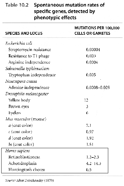
Deleterious
alleles are maintained by recurrent mutation.
A stable
equilibrium![]() (where
(where ![]() q
= 0) is reached
q
= 0) is reached
when the rate of replacement (by mutation)
balances the rate of removal (by selection).
µ
=
frequency of new mutant alleles per locus per generation
typical µ =
10-6: 1 in 1,000,000 gametes has
new
mutant
_____
then ![]() =
=![]() (µ
/ s) [see derivation]
(µ
/ s) [see derivation]
Ex.: For a recessive lethal allele (s = 1) with a
mutation
rate of µ = 10-6
then ![]() = û
=
= û
= ![]() (10-6
/ 1.0) = 0.001
(10-6
/ 1.0) = 0.001
mutational
genetic
load
Lowering selection against alleles increases their frequency.
Medical intervention has increased the frequency of heritable
conditions
in Homo (e.g., diabetes, myopia)
Eugenics:
modification of human condition by selective breeding
'positive eugenics': encouraging people with "good genes" to
breed
'negative eugenics': discouraging people with 'bad genes'' from
breeding
e.g., immigration control, compulsory sterilization
[See: S. J. Gould, "The
Mismeasure of Man"]
Is
eugenics effective at reducing frequency of deleterious alleles?
What proportion of 'deleterious alleles' are found in heterozygous
carriers?
(2pq)
/ 2q2 = p/q ![]() 1/q
(if q << 1)
1/q
(if q << 1)
if s = 1 as above, ratio is 1000 / 1 : most of
variation
is in heterozygotes,
not subject to selection
Directional
selection is balanced by influx of 'immigrant' alleles;
a stable 'equilibrium' can be reached iff migration rate constant.
Consider an island adjacent to a
mainland,
with unidirectional
migration to the island.
The fitness values of the AA, AB,
and BB genotypes differ in the two environments,
so that
the allele frequencies differ between the mainland (qm)
and the island (qi).
| AA | AB | BB | ||
|
|
W0 | W1 | W2 | q |
| Island | 1 | 1-t | 1-2t | qi |
| Mainland | 0 | 0 | 1 | qm |
B has high fitness on
mainland,
and low fitness on island.
[For this model only,
allele A is semi-dominant to allele B,
so we use t for the selection coefficient to avoid confusion]
m
=
freq. of new migrants (with qm)
as fraction of residents (with qi)
if m
<< t qi
= (m / t)(qm)
[see derivation]
Gene flow can hinder optimal adaptation of a population to local conditions.
Ex: Water
snakes (Natrix sipedon) live on islands
in Lake Erie (Camin & Ehrlich 1958)
Island
Natrix mostly unbanded; on adjacent mainland, all
banded.
Banded snakes are non-cryptic on limestone islands, eaten by gulls
Suppose A = unbanded B
= banded [AB are intermediate]
Let qm =
1.0
["B" allele is fixed on mainland]
m = 0.05 [5% of island snakes are new
migrants]
t = 0.5 so W2
= 0 ["Banded" trait is lethal on island]
then qi =
(0.05/0.5)(1)
= 0.05
and Hexp = 2pq =
(2)(0.95)(0.05) ![]() 10%
10%
i.e, about 10% of snakes show intermediate banding, despite
strong
selection
=> Recurrent migration can maintain a disadvantageous trait at high
frequency.
Inbreeding
is the mating of (close) relatives
or, mating of individuals with at least one common ancestor
F (Inbreeding
Coefficient) = prob. of "identity
by descent":
Expectation that two alleles
in an individual are
exact genetic copies of an allele in
the
common ancestor
or, proportion of population with two
alleles identical by descent
This is determined by the consanguinity (relatedness) of parents.
Inbreeding
reduces
Hexp by a proportion F
(& increases the proportion of homozygotes). [see
derivation]
f(AB) = 2pq (1-F)
f(BB) = q2 + Fpq
f(AA) = p2 + Fpq
Inbreeding
affects genotype proportions,
inbreeding does not affect allele frequencies.
Inbreeding
increases the frequency of individuals
with deleterious recessive genetic diseases by F/q [see derivation]
Ex.: if q = 10-3 and F
= 0.10 , F/q = 100
=> 100-fold increase in f(BB) births
Inbreeding coefficient of a population can be estimated from experimental data:
F = ( 2pq - Hobs ) / 2pq [see derivation]
Ex.: Selander (1970) studied structure of Mus house mice living in chicken sheds in Texas|
|
|
|
|
|
|
|
|
|
|
|
|
|
|
|
& q = 0.374 + (1/2)(0.400) = 0.574
Then F = (0.489 - 0.400) /
(0.489)
= 0.182
which is
intermediate
between Ffull-sib =
0.250
& F1st-cousin = 0.125
=> Mice live
in small
family groups with close inbreeding
[This is typical for small mammals]
However, in combination with natural selection, inbreeding can be
"advantageous":
increases rate of evolution in the long-term (q![]() 0 more quickly)
0 more quickly)
deleterious alleles are eliminated more quickly.
increases phenotypic variance (homozygotes are more
common).
advantageous alleles are also reinforced in homozygous form
Genetic
Drift is stochastic ![]() q
[unpredictable,
random]
q
[unpredictable,
random]
(cf. deterministic ![]() q
[predictable,
due to selection, mutation, migration)
q
[predictable,
due to selection, mutation, migration)
Sewall Wright (1889 - 1989): "Evolution and the Genetics of Populations"
Stochastic ![]() q
is greater than deterministic
q
is greater than deterministic ![]() q
in small populations:
q
in small populations:
allele frequencies drift more in 'small' than 'large' populations.
Drift is
most noticeable if s ![]() 0,
and/or N small (< 10) [N
0,
and/or N small (< 10) [N ![]() 1/s]
1/s]
q
drifts between generations (variation decreases within
populations
over time) [];
eventually, allele is lost (q = 0) or fixed (q
= 1) (50:50 odds)
Ex:
[Demonstration
#3]
[Try: q = 0.5, W0 = W1 = W2 = 1.0, and N = 10, 50, 200, 1000;
repeat 10 trials each, note q at
endpoint]
q
drifts among populations (variation
increases
among populations over time);
eventually, half lose the allele, half fix it.
**=> Variation is 'fixed' or 'lost' & populations will diverge by chance <=**
Evolutionary
significance:
"Gambler's Dilemma" : if you play
long enough, you win or lose
everything.
All populations are finite: many are very small,
somewhere
or sometime.
Evolution occurs on vast time scales: "one in a million chance"
is a certainty.
Reproductive success of individuals in variable: "The race
is
not to the swift ..."
What happens in the really long run?
Effective
Population Size (Ne)
= size of an 'ideal'
population with same genetic variation (measured
as
H)
as the observed 'real' population.
= The 'real' population
behaves evolutionarily like one of size Ne
:
e.g., the population will
drift like one of size Ne
loosely,
the
number of breeding individuals in the population
Consider three special cases where Ne < or << Nobs [the 'count' of individuals]:
(1) Unequal sex ratio
Ne = (4)(Nm)(Nf) /
(Nm + Nf)
where Nm & Nf are numbers of
breeding
males & females, respectively.
"harem" structures in mammals (Nm << Nf)
Ex.: if Nm = 1 "alpha male" and Nf
= 200
then Ne = (4)(1)(200)/(1 +
200) ![]() 4
4
A single male elephant
seal (Mirounga)
does most of the breeding
Elephant seals have very low genetic variation
eusocial (colonial)
insects
like ant & bees (Nf << Nm)
Ex.: if Nf = 1 "queen" and Nm=
1,000 drones
then Ne = (4)(1)(1,000)/(1 +
1,000) ![]() 4
4
Hives are like single small families
(2) Unequal
reproductive success
In stable population, Noffspring/parent
= 1
"Random" reproduction follows
Poisson
distribution
(N = 1 ![]() 1)
1)
(some parents have 0, most have 1, some have 2, a few have 3 or more)
| X | Ne = | Reproductive strategy | |
| 1 | 1 | Nobs | Breeding success is random |
| 1 | 0 | 2 x Nobs | A zoo-breeding strategy |
| 1 | >1 | < Nobs | K-strategy, as in Homo |
| 1 | >>1 | << Nobs | r-strategy, as in Gadus |
(3) Population size variation over time
Ne = harmonic mean
of N = inverse of arithmetic mean of inverses
[a harmonic mean is much closer to lowest value in series]
n
Ne = n / [ ![]() (1/Ni)
] where Ni = pop size in i th
generation
(1/Ni)
] where Ni = pop size in i th
generation
i=1
Populations
exist in changing environments:
Populations are unlikely to be stable over very long periods of time
10-2 forest fire / 10-3 flood / 10-4
ice
age
Ex.: if typical N = 1,000,000 & every 100th
generation
N
= 10 :
then Ne = (100) / [(99)(10-6) +
(1)(1/10)] ![]() 100 / 0.1 = 1,000
100 / 0.1 = 1,000
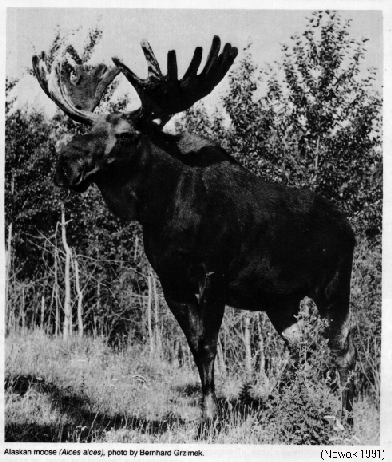
Founder
Effect & Bottlenecks:
Populations are started by (very) small number of individuals,
or undergo dramatic reduction in size.
Ex.: Origin of Newfoundland moose (Alces):
2 bulls + 2 cows at Howley in 1904
[1 bull + 1 cow at Gander in 1878 didn't succeed].
Population
cycles: Hudson
Bay Co. trapping
records (Elton 1925)
Population densities of lynx, hare, muskrat cycle over several orders
of
magnitude
Lynx cycle appears to "chase" hare cycle
The effect of drift on genetic variation in populations
Larger populations are more variable (higher H) than
smaller
if s = 0: H reflects balance between loss of
alleles
by drift
and replacement by mutation
H = (4Neµ) / (4Neµ + 1)
Ex.: if µ= 10-7 & Ne = 106 then Neµ = 1 and Hexp = (0.4)/(0.4 + 1) = 0.29
But
typical
Hobs ![]() 0.20 which suggests Ne
0.20 which suggests Ne ![]() 105
105
Most natural populations have a much
smaller
effective size than their typically observed size.
Stochastic effects may be as or more important than deterministic
processes
in evolution.