The Chi-Square Test for Hardy-Weinberg Expectations of SNP data
(1) For a locus with an A / G SNP polymorphism,
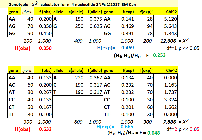
given the observed genotype counts that total to 200,
the f(obs) of each genotype is (given) / (total). The
count of alleles c(alleles) is then two for
each homozygote plus one for each heterozygote, for
example c(A) = (2)(40) + 70 = 150. Noting that the
number of alleles is twice the number of genotypes, the
frequency of alleles f(allele) is f(A) = 150 / 400 =
0.375. Then, f(G) = 250 / 400 = 0.625 or (1 - f(A))
= (1 - 0.375). Calculate the expected
genotype frequencies from these observed
allele frequencies: if p = f(A) and q = f(G),
then p2 = f(AA),
2pq = f(AG), and q2
= f(GG). Expected genotype counts
in each case are then (frequency) X (total observed).
The proportional deficiency of heterozygotes (F) can be calculated here from knowledge of the observed heterozygosity (0.350) and the expected heterozygosity (calculated as 2pq = (2) (0.375)(0.625) = 0.469, thus F = (0.350 - 0.469) / 0.469 = 0.253. A deficiency of heterozygotes is also called the Inbreeding Coefficient (F), if it is attributable to selective union of similar gametes, and (or) selective mating of similar genotypes. The theory of this is dealt with elsewhere.
Calculate the Chi-Square deviation (X2) contributed by each genotype as the difference between the observed and expected counts, divided by the expected count, quantity squared. For AA, (AAobs - AAexp)2 / (AAexp) = (40 - 28)2 / (40) = 5.120. The calculation is repeated for each genotype, and the Chi-Square value X2 for the test is the sum over all genotypes, in this case 12.606.
(2) To evaluate the statistical significance of this value, it is necessary to know the number of degrees of freedom (df) in the experimental data, which is reported and evaluated along with the result. In general, the df in any experiment is one less than the number of categories compared, (n-1). The principle is that, if you know you looked at n experimental results that could have fallen into any of three categories a b c, the value of the first category a can be anything (up to n), and the value of the second category b can be anything up to (n-a). Having determined a and b, the third value is now pre-determined: c = (n - a - b). So, only two of the three values are free to vary.
For diploid genotypic data with two alleles A & G and three genotype counts AA, AG, & GG, this would suggest df = 2 in a test of two sets of observed data. However, given f(A), the expected frequencies for all three genotypes are automatically determined as f(AA), f[(A)(1-A)], & f[(1-A)(1-A)], thus df = 1 in a test of observed data versus expectations for those data. Note a higher df requires a greater departure of observed from expected for statistical significance.
(3) The same principles apply to calculations for any three-allele (A / C / T for example), or four-allele (A / C / G / T) SNP polymorphism, with two and three degrees of freedom, respectively.
The Bio4250 Excel workbook includes a spreadsheet for calculation of SNP polymorphism for 2, 3, or 4 alleles.
Four further points with respect to SNP data should be kept in mind.
(4) Calculation of expected genotype counts from observed frequency data often results in expectations of non-integral numbers. Avoid 'fractional individuals'. If we were testing for a 3:1 genotypic ratio among 17 individuals, we cannot expect to see 12.75 and 4.25, so we round to the closest integer, here 13 and 4, which still adds to 17. This is applicable to the multiple-category data above. A related problem arises when, among 18 individuals, calculated expectations are 13.5 and 4.5: if we round both to 13 and 4, we are shy one expected and the test calculation is biased. One convention is to round one or the other expectation against the trend seen in the data. That is, if we have a 3:1 hypothesis and observe 15 & 3, we round the expectations to 14 & 4. If we observed 12 & 6, we round the expectation to 13 & 5. This is not 'massaging' the data: the rounding reduces the likelihood of obtaining a significant result due to a computational bias, and increases the confidence in the result.
(5) Chi-square calculations must always be performed with count data, not frequencies or percentages. Because it squares the magnitude of the deviation, X2 values are heavily influenced by the absolute magnitude of the numbers. For 0.6 & 0.4 observed versus 0.5 & 0.5 expected, X2 = 0.12 / 0.5 + (-0.1)2 / 0.5 = 0.02 / 0.5 = 0.04 ns, whereas with 60 & 40 versus 50 & 50 expected, X2 = 102 / 50 + (-10)2 / 50 = 200 / 50 = 4.0* , and with 600 & 400 versus 500 & 500 expected X2 = 1002 / 500 + (-100)2 / 500 = 20,000 / 500 = 40.0***. The proportional deviation is the same in each case (20%), but when the actual deviation is squared, and contributes much for strongly to X2 as n increases. This is also a reminder that larger samples sizes produce experiments with greater statistical power.
(6) One school of statistical genetics says that, for diploid genotypic data with two alleles A & G and three genotypes AA, AG, & GG, if we know q = f(G), then f(A) = (1-q), and f(AA) = (1-q)2, f(AG) = (2)(1-q)(q) and f(GG) = q2. Therefore, the expected values of the three genotype categories are pre-determined by the expected value of either of the two allele frequencies, which per-determines the other, and therefore df = 2 - 1. Then, for nucleotide or other allelic data, df = n-1 where n = # of alleles. IMO, because the observed rather than the expected genotypic proportions are being tested, df should be calculated from the number of observed classes, as above.
(7) The method shown here is Pearson's Chi-square test procedure, which is the classical method taught in genetics courses for genotypic and other comparisons. It is now appreciated that this test over-estimates the significance of any observed deviation, especially for small cell values. The G-Test can be used for the same purpose, and is included in the Biol4250 Excel workbook. Each cell value X in the two-column data matrix is transformed as X' = XlnX. The statistical test is then a Row-by-Column (RxC) Test of Independence on the transformed data. The significance of the test is obtained from the Chi-Square table. The G-test has a number of advantages, notably that it is unaffected by sample size, can be estimated from fractional expectations, and results from individual tests are additive to the result for the total test.
[Historical note: The advantages of the G-Test with respect to the Chi-Square Test were appreciated before its routine use. Long before the advent of personal computers, electronic calculators, and before the routine availability of digital mainframe computers, calculation of XlnX required printed tables of the values of lnX and (or) pre-calculated XlnX, and manual entry of these values onto the dials of mechanical calculating machines. For any sizeable calculation, this was complicated and tedious. See for example the 1st (1969) edition of Sokal & Rohlf "Biometry" and the accompanying "Statistical Tables" for some context].
Text material © 2022 by Steven M. Carr