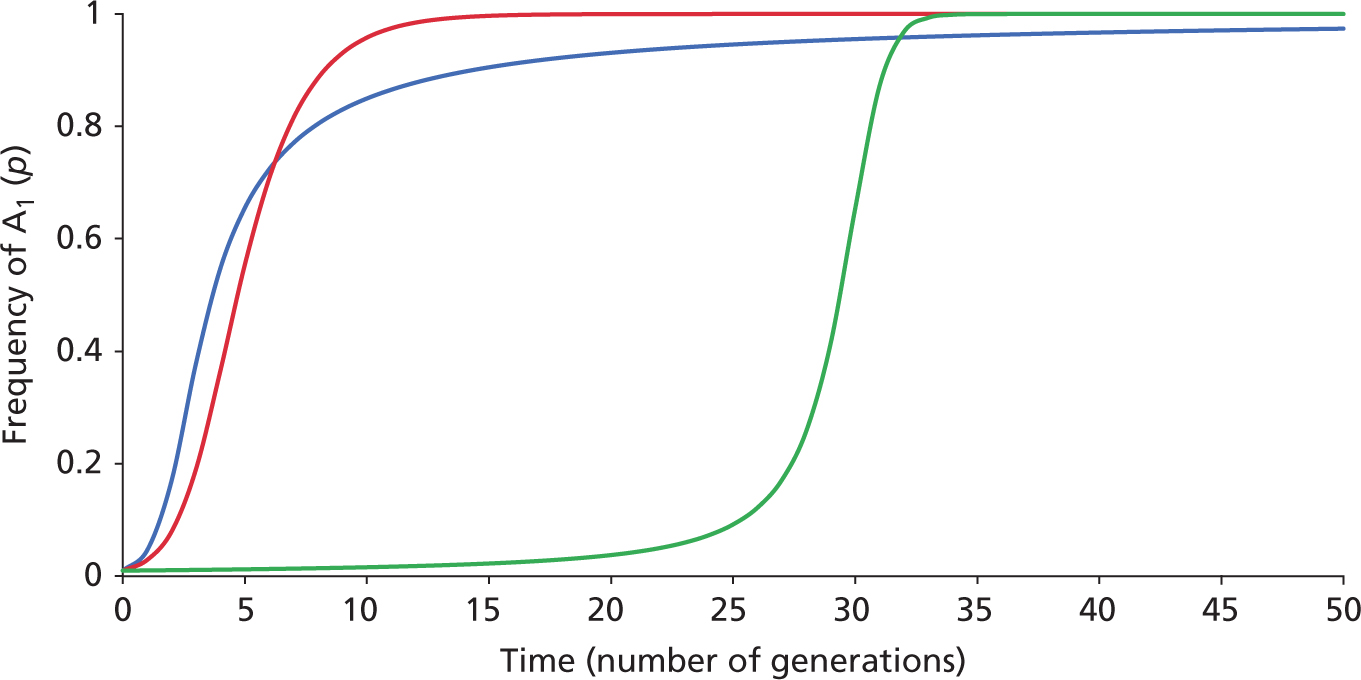
Change in frequency
of a rare allele under Positive
Directional Selection
Dominant, Additive Semi-Dominant, & Recessive cases
In a single-locus model
with two alleles A1 and A2,
initial p = f(A1)
= 0.001. The three curves
trace f(A1)
over time for three
modes of dominance.
The Blue curve
shows the case of dominance of
W11 to W12 (W11
= W12 = 1.0). The Red curve shows an additive (semi-dominance) model, in
which each W2 allele
decreases dW = 0.4, such that W12
= 1.0 - 0.4 = 0.6., and W22
= 1.0 - (0.4+0.4) = 0.2. The Green curve shows
the case where
W22
is recessive to
W12
(W12
= 0.2). The difference between
the shapes of the curves reflects how mean population fitness
(![]() )
varies as f(A1)
)
varies as f(A1) ![]() 1.0.
1.0.
NB: The dominance relationships
of any two alleles at a locus are fixed genetically.
The graph also shows the fate of a common allele
under negative directional selection, IF Y-axis values are inverted
top to bottom (1 ![]() 0) and labelled
f(A2) = q. That is, the
behaviors of advantageous and disadvantageous alleles
are complementary for any particular dominance
model.
0) and labelled
f(A2) = q. That is, the
behaviors of advantageous and disadvantageous alleles
are complementary for any particular dominance
model.
The principles presented in
this graph will be explored in greater depth in the laboratory
exercises for Natural Selection.
HOMEWORK: Demonstrate that these curves can be obtained from similar selection coefficient values in the Hardy - Weinberg selection programs GSM in Excel, or natsel in Python. Important Note: REMEMBER that this is a graph of p, rather than q as elsewhere in these notes, or in the two programs.