Deterministic change of an advantageous allele
when Dominance of Fitness is Dominant, Recessive, or Additive
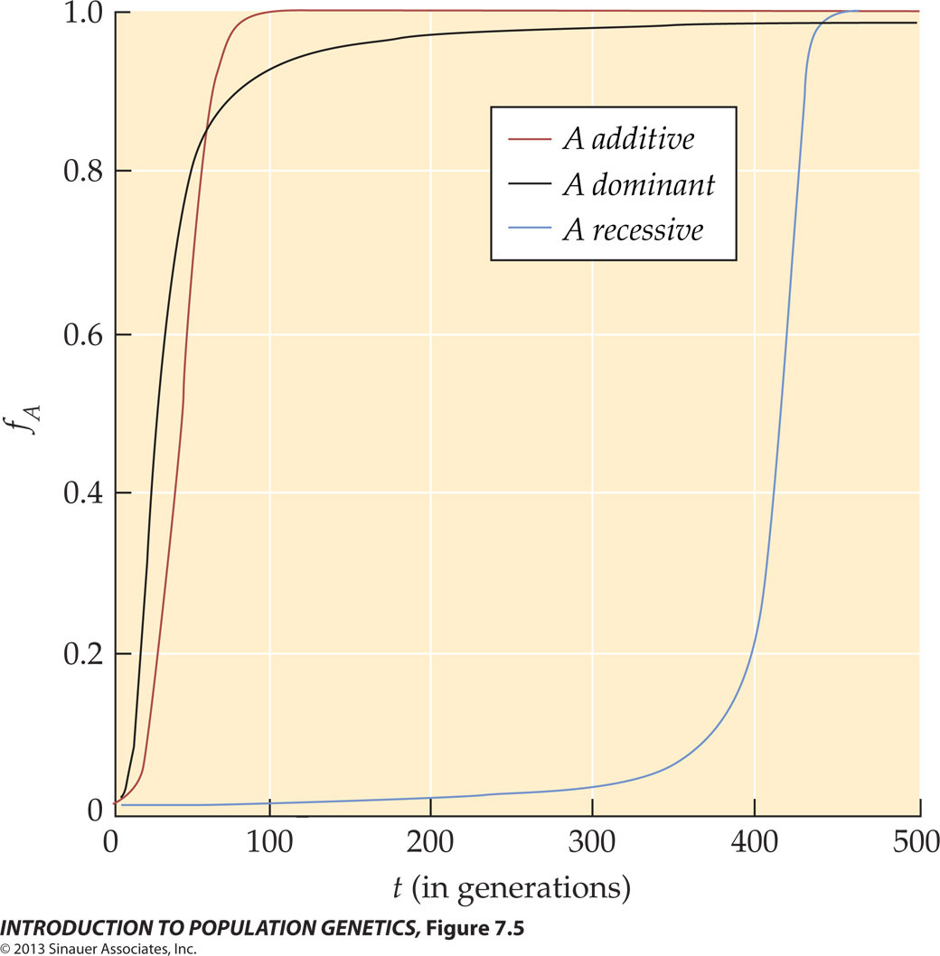
The graphs here summarize the expected results obtained
for particular values as stated below. Use the Excel spreadsheet models
to model these same conditions, as well as others.
f(A)
is plotted for a locus with two alleles A
and B. Dominance of
Fitness is defined by whether A is dominant,
recessive, or additive ("semi-dominant")
with respect to B. In a model where allele A is always at
a selective advantage to B, these
models correspond to WAB = 1.0,
0.8, or 0.9, respectively. The additive
model assumes that each B allele reduces
fitness by a fraction s = 0.1, so WAA
= 1.0, WAB
= (1-s), and WBB
= (1-2s).
The selection equation here is deterministic: the frequency of the advantageous allele A will always increase, even from a very low initial value f(A) = 0.01 as shown.
(I) When A is dominant , f(A) increases very quickly, and approaches fixation (f(A) = 1) asymptotically, because the recessive allele can never be completely eliminated.
(II) When A is recessive, f(A) increases very slowly, because the advantageous genotype is initially very rare [ f(AA)0 = 0.0001 & f(AB)0 ~ 0.02, so f('A' ~ 0.02) ], and even when f(A)350 = 0.1, f(AA)350 = 0.01 & f(AB)350 ~ 0.18 so that f('A' ~ 0.2). Allele A will eventually become fixed because B is always exposed to selection.
(III) When A is additive [i.e., the effect of B is additive], f(A) increases quickly, but not so quickly as in the simple dominant case, because there is selection against the B allele in the heterozygous AB genotype. In this case, unlike the strict dominance case (I), the A allele can go to fixation, because as in (II) B is always exposed to selection.
Compare this diagram with (SR2019 4.3).
Text material © 2020 by Steven M. Carr