Critical values & degrees of freedom of the
 2 distribution
The critical
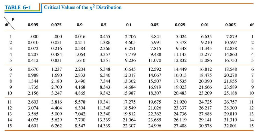
value of a statistical test is the
numerical value at which an observed result is statistically significant
at some pre-determined degree of probability.
For example, for a 2 test with one df = 1, the table shows
that if 2 >
3.841, the observed result would be expected to occur
by chance less than one time in twenty, that it, is has a
probability p < 0.05. If the
significance level of the test had been set at p = 0.05, the observed
results is said to be statistically
significant.
Where the observed result exceeds the critical value for p = 0.01, the result is
sometimes said to be highly
significant. Strictly, the significance level is set
a priori (before the
experiment is carried out), and any result is either
significant or non-signficant at that level.
The simplest kind of statistical test has only two possible outcomes ("either / or") and is also called a single-classification test. In such a test, the number of events in the first category automatically determines the number in the second. Because of this, the experiment is said to have only a single degree of freedom, or df = 1. For a more complicated experiment with C possible categories of outcome for N events, the number of events that can fall into any of the first C-1 categories can vary freely. The number of events in the last category must make the total add up to N, and is thus constrained. The experimental outcome has lost one degree of freedom, and in general df = (# of possible outcomes - 1).
2 test with one df = 1, the table shows
that if 2 >
3.841, the observed result would be expected to occur
by chance less than one time in twenty, that it, is has a
probability p < 0.05. If the
significance level of the test had been set at p = 0.05, the observed
results is said to be statistically
significant.
Where the observed result exceeds the critical value for p = 0.01, the result is
sometimes said to be highly
significant. Strictly, the significance level is set
a priori (before the
experiment is carried out), and any result is either
significant or non-signficant at that level.The simplest kind of statistical test has only two possible outcomes ("either / or") and is also called a single-classification test. In such a test, the number of events in the first category automatically determines the number in the second. Because of this, the experiment is said to have only a single degree of freedom, or df = 1. For a more complicated experiment with C possible categories of outcome for N events, the number of events that can fall into any of the first C-1 categories can vary freely. The number of events in the last category must make the total add up to N, and is thus constrained. The experimental outcome has lost one degree of freedom, and in general df = (# of possible outcomes - 1).