F-Statistics as measures of genetic population structure
A numerical example
Previously, we used F to measure the deficiency of heterozygotes due to either mating of closely-related individuals (inbreeding) within local populations, or differences in allele frequencies among local populations (Wahlund Effect). We now generalize the concept to estimate genetic population structure. Suppose a global species occurs as a series of local populations. Local populations may differ in allele frequencies. If these local populations are structured such that they do not exchange individuals uniformly (they are not panmictic), then individuals are more likely to mate with neighbors in the same local population. Local populations are then more likely to comprise related individuals. If structure varies among populations, then populations themselves will be more or less related. Structure here may be geographic (more distant population are more dissimilar), ecological (populations in different habitats are dissimilar), or historical (recently founded populations may show founder and drift effects). F-statistics are particularly useful when the degree of geographic, ecological, or historical structure is unknown, but can be formulated as hypotheses to be tested.
Heterozygosity and F-statistics can also be thought of as random-draw-&-replacement experiments. Draw an allele at random from any particular sub-population, note and replace it. What is the expectation that a second allele drawn from the same sub-population will be different? That is, what is the chance of drawing a heterozygous pair? Repeat this for all sub-populations. What is the expectation of heterozygosity if the second allele is drawn from a different sub-population? What if this experiment is repeated with alleles drawn from different pairs of sub-populations? From all possible pairs of sub-populations? Expectations differ for each of these experiments, according to the heterogeneity of allele and genotype frequencies measured as H among populations. Genetic structure will always reduce the expectation of heterozygosity as calculated from the global allele frequency. The deficiency can be expressed as F calculated at different levels of population structure.
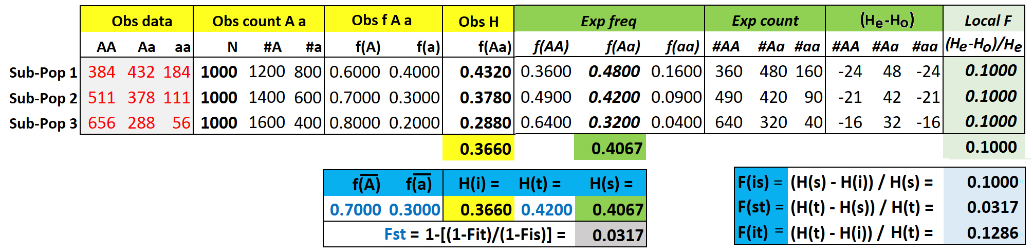
Consider a simple model of individuals distributed among three sub-populations of a global population, with observed genotype counts for each sub-population as indicated in the grey box. Based on these counts, we wish to compare the expected vs observed heterozygosity at each of these three levels of population structure. The population sizes of the three sub-populations are equal (N = 1000). This simplifies the calculations, otherwise contributions from sub-population of different size must be weighted by sample size, and use of a round number makes the math easier.
From the genotype data for each sub-population, observed allele counts #A & #a and frequencies f(A) & f(a) are easily calculated in the usual manner. Expected genotype counts & frequencies are then easily calculated from the observed allele frequencies, for example Hexp = (2)(fA)(fa). Global fA (
Heterozygosity indices Hi, Hs, and Ht are simply H, calculated at different levels of the population structure. With equal N, these are easily calculated from the bold values in the table above, as
Hi = mean of observed f(Aa) = (0.432 + 0.378 + 0.288) / 3 = 0.3660
This is the observed probability of heterozygosity for an individual drawn at random from any sub-population.
Hs = mean of expected f(Aa) = (0.480 + 0.420 + 0.320) / 3 = 0.4067
This is the expectation of heterozygosity for two alleles drawn at random from any pair of sub-populations.
Hi and Hs differ when sub-populations have different genetic structures. The difference is a measure of genetic population structure.
Ht = Expected "global" heterozygosity is calculated as
as calculated in the second box, lower left. This is simply the global (total) expectation of heterozygosity based on the observed total allele frequencies.
This deficiency of heterozygotes can be expressed as a set of three F-statistics, which are hierarchical versions of H, at each level with respect to the next more inclusive level. These are easily calculated with equal N across sub-populations. Recall that F and H for any single population are related as F = (He - Ho) / He = 1 - (Ho / (He). The analogous calculations are shown in the third box, lower right:
Fis = mean deficiency of observed heterozygotes among individuals with respect to that expected across sub-populations.
In this example, where local F is the same across sub-populations, Fis is equivalent to local F.
Fit = mean deficiency of observed heterozygotes among individuals with respect to that expected for the total population,
which in equivalent to Wahlund Effect, when allele frequencies differ across sub-populations.
Fst = mean deficiency of expected heterozygotes among sub-populations with respect to that expected for the total population,
which in this case is a measure of population differentiation among sub-populations with respect to the total.
Fst in various forms is the most widely used descriptor of population genetic structure with diploid data (nuclear DNA sequences, or allozymes). The concept can be extended to multiple sub-populations within a population, or multiple population levels within species. Equivalent measures can be calculated for haploid data (mtDNA).
HOMEWORK: Two ways of calculating FST are shown, in terms of FIT & FIS or HT & HS. SHOW that the two calculations are equivalent.
Figures & Text material © 2025 by Steven M. Carr