Natural Selection on semi- & incompletely dominant phenotypes with Additive & Genic fitness
In classical genetics, if the phenotype
of the AB genotype is precisely intermediate
between those of the two homozygous genotypes AA and
BB, A and B are described as semi-dominant. If
the phenotype of the AB genotype is intermediate
between AA & BB, but closer to that of
the AA than the AB genotype, A is
described as incompletely dominant
to B. If AB is closer to BB, then B
is the incompletely dominant allele.
A numerical example of semi-dominance occurs when genotypes AA, AB, & BB are assigned fitness values of W0 = 0.2, W1 = 0.4, and W2 = 1.0. BB has the highest fitness: with selection coefficient s = 0.4, the fitness values would be written as WAA = (1-2s), WAB = (1 - s), and WBB = (1). Each A allele contributes an additive selective disadvantage of s = 0.4, so that an AA homozygote is at twice the disadvantage of the AB heterozygote.
In the table below, fitness in either Additive of Genic fitness is (1 - s). Note that if s > 0.5, the additive fitness of AA homozygotes W0 < 0 and therefore undefined. For s < 0.5, fitness is positive though initially low.
Note once again that, if B is incompletely dominant to A, it is not because B has superior fitness (and might be said to "dominate" the other allele), but because the AB phenotype is intermediate between that of the AA and BB. Genetic dominance is a genotypic, not a phenotypic, relationship.Nor does it make a difference if f(B) > f(A), or f(B) < f(A) such that one allele could be to 'predominate' the other.
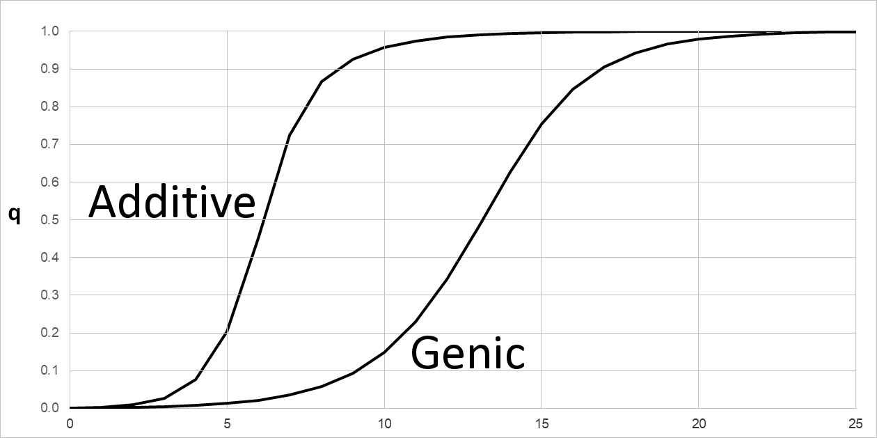
Compare this model with that for Genic (Multiplicative) fitness. Again, let initial q = f(B) = 0.001. Using the notation of selection coefficients with s = 0.4 as above, WBB = (1), WAB = (1 - s), and WAA = (1 - s)(1 - s) = (1 - s)2 , so W2 = 1.0 , W1 = 0.4, and W0 = 0.36. That is, each A allele reduces fitness by a factor of (1 - s). The fitness effect of a single allele is (1 - s) in either model. However, the two models make very different predictions about dq over the range 0.1 ~ s ~ 0.5. At smaller values of s, the expected difference between models becomes negligible and too small to be measured. This is because genic fitness (1 - s)2 = 1 - 2s + s2 ~ (1 - 2s) as in additive fitness, when s2 << 2s or s << 2.
Simple additive dominance may be typical at many gene loci, where the phenotype is a consequence of equal expression by both alleles. For example, each allele at a protein-coding locus may contribute half the total amount of gene product. This might explain so-called "null alleles" in protein electrophoresis, in which one allele produces no product, and only one band is seen. The other, functional allele that produces 50% of the expected gene product may (or may not) provide sufficient enzyme product for standard phenotypic expression. Incomplete genic dominance may be typical at gene loci, where the phenotype is (much) more strongly influenced by one allele than the other. For example, given a null allele that produces no gene product, the standard allele may be "up-regulated" so that the amount of gene product in the AB heterozygote is (much) closer to that of the AA homozygote.
It remains a major point of contention what fraction of heterozygous allelic variation detected originally by protein electrophoresis and (or) nowadays by DNA sequencing has any measurable effect on the observed phenotype relative to that of the homozygotes, as is clear from the math above. The so-called "Neutralist - Selectionist" controversy will be discussed elsewhere in the course.
HOMEWORK:
(1) For an initial qo = f(B) = 0.000001 OR AS INSTRUCTED, use the GSM worksheet in Excel to run the (1) Additive and (2) Genic selection models for s≼ 0.5
(2) For an initial qo = f(B) = 0.000001 OR AS INSTRUCTED, use the GSM Worksheet to run the Semi Dominance model.
(3) Can you use the GSM to simulate Haploid Selection? Why or why not?
A numerical example of semi-dominance occurs when genotypes AA, AB, & BB are assigned fitness values of W0 = 0.2, W1 = 0.4, and W2 = 1.0. BB has the highest fitness: with selection coefficient s = 0.4, the fitness values would be written as WAA = (1-2s), WAB = (1 - s), and WBB = (1). Each A allele contributes an additive selective disadvantage of s = 0.4, so that an AA homozygote is at twice the disadvantage of the AB heterozygote.
In the table below, fitness in either Additive of Genic fitness is (1 - s). Note that if s > 0.5, the additive fitness of AA homozygotes W0 < 0 and therefore undefined. For s < 0.5, fitness is positive though initially low.
Note once again that, if B is incompletely dominant to A, it is not because B has superior fitness (and might be said to "dominate" the other allele), but because the AB phenotype is intermediate between that of the AA and BB. Genetic dominance is a genotypic, not a phenotypic, relationship.Nor does it make a difference if f(B) > f(A), or f(B) < f(A) such that one allele could be to 'predominate' the other.
Compare this model with that for Genic (Multiplicative) fitness. Again, let initial q = f(B) = 0.001. Using the notation of selection coefficients with s = 0.4 as above, WBB = (1), WAB = (1 - s), and WAA = (1 - s)(1 - s) = (1 - s)2 , so W2 = 1.0 , W1 = 0.4, and W0 = 0.36. That is, each A allele reduces fitness by a factor of (1 - s). The fitness effect of a single allele is (1 - s) in either model. However, the two models make very different predictions about dq over the range 0.1 ~ s ~ 0.5. At smaller values of s, the expected difference between models becomes negligible and too small to be measured. This is because genic fitness (1 - s)2 = 1 - 2s + s2 ~ (1 - 2s) as in additive fitness, when s2 << 2s or s << 2.
Simple additive dominance may be typical at many gene loci, where the phenotype is a consequence of equal expression by both alleles. For example, each allele at a protein-coding locus may contribute half the total amount of gene product. This might explain so-called "null alleles" in protein electrophoresis, in which one allele produces no product, and only one band is seen. The other, functional allele that produces 50% of the expected gene product may (or may not) provide sufficient enzyme product for standard phenotypic expression. Incomplete genic dominance may be typical at gene loci, where the phenotype is (much) more strongly influenced by one allele than the other. For example, given a null allele that produces no gene product, the standard allele may be "up-regulated" so that the amount of gene product in the AB heterozygote is (much) closer to that of the AA homozygote.
It remains a major point of contention what fraction of heterozygous allelic variation detected originally by protein electrophoresis and (or) nowadays by DNA sequencing has any measurable effect on the observed phenotype relative to that of the homozygotes, as is clear from the math above. The so-called "Neutralist - Selectionist" controversy will be discussed elsewhere in the course.
HOMEWORK:
(1) For an initial qo = f(B) = 0.000001 OR AS INSTRUCTED, use the GSM worksheet in Excel to run the (1) Additive and (2) Genic selection models for s
(2) For an initial qo = f(B) = 0.000001 OR AS INSTRUCTED, use the GSM Worksheet to run the Semi Dominance model.
(3) Can you use the GSM to simulate Haploid Selection? Why or why not?
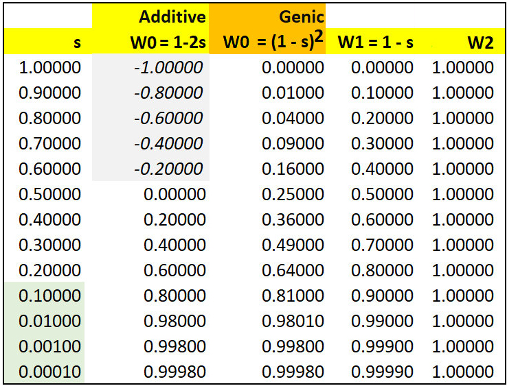
Table & text material © 2025 by Steven M. Carr