 2 = µ). The probability
P of observing Y events in a Poisson-distributed
process with a mean = u is
2 = µ). The probability
P of observing Y events in a Poisson-distributed
process with a mean = u is
| µ | N |
0 | 1 | 2 | 3 | 4 | 5 | not 0 | >(0+1) | |
| 0.100 | 90.5% | 9.0% | 0.5% | 0.0% | 0.0% | 0.0% | 9.5% | 0.5% | |
| 0.125 | 88.2% | 11.0% | 0.7% | 0.0% | 0.0% | 0.0% | 11.8% | 0.7% | |
| 0.250 | 77.9% | 19.5% | 2.4% | 0.2% | 0.0% | 0.0% | 22.1% | 2.6% | |
| 0.500 | 60.7% | 30.3% | 7.6% | 1.3% | 0.2% | 0.0% | 39.3% | 9.0% | |
| 0.750 | 47.2% | 35.4% | 13.3% | 3.3% | 0.6% | 0.1% | 52.8% | 17.3% | |
| 1.000 | 36.8% | 36.8% | 18.4% | 6.1% | 1.5% | 0.3% | 63.2% | 26.4% |
The Poisson distribution is a
special case of the binomial distribution
that
applies
where the phenomenon under study occurs as rare, discrete
events. The characteristic statistical property of a Poisson
distribution is that the variance equals the mean
(2 = µ). The probability
P of observing Y events in a Poisson-distributed
process with a mean = u is
P(Y; u) =
e-u uY /
Y!
(1) In a study of
the distribution of a rare plant among a number of standardized
quadrat plots, a majority of plots may be expected to contain no
specimens, a smaller number a single plant, and still smaller
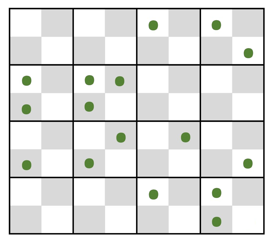
numbers two, three, or more plants. If 16 plants are
distributed randomly over the 4x4 checkerboard quadrat
below (mean µ = 1),
the table shows that a random Poisson distribution over the cells
should produce "0" and "1" classes at 37%
each, a "2" class at 18%,
the "3" class at 6%, and
the more frequent classes will take up the remaining 2%. In the
example, there are16 plants distributed as 6, 5, 4, and 1 cells
with 0, 1, 2, and 3 plants, respectively. A Chi-square test
that conforms to expected µ
= 1 ± 1 indicate that the rare plant is distributed
randomly.
(2) The Poisson can simplify analysis of a simple "either
/ or" data set. In the quadrat example with µ = 1, the Poisson
random expectation is that 37% of the quadrat plots will
be unoccupied (0) and the remaining 63%
occupied.(not 0). In a 2x2 test, a
significant excess of
empty cells means the plants are clumped, and a
significant deficiency means
the plant distribution is more uniform. The
former might occur if suitable soil is patchily distributed,
the latter if plants space themselves out to avoid
competition for resources.
(3) Conversely, if it assumed that events occur randomly
the number of observed events can be used to estimate
the actual number of events. For example, suppose I am
throwing rocks at a building with 100 windows. Initially, a good
estimate of the number of thrown rocks is the count of broken
windows. After a bit, this count is an underestimate,
because a rock that goes through a window already broken will
not be counted. We can then apply a Poisson Correction
to estimate the number of multiple hits from the zero
class. From the above, the expected probability of the
zero class (P0) simplifies
to
P0
= e-u u0
/ 0! = e-u
where u = corrected fraction
of hits. For example, if 39 out of 100 windows
are broken, then 61 are
unbroken, and P0 = 0.61 =
e-u
Taking the minus natural log of both sides
gives u = - ln(0.61) / 1 = 0.50
That is, the
actual number of "hits" is (100)(0.50) = 50 rather
than the observed 39 broken windows a correction of 11
/ 39 = 0.28. (From the table above, note that this
correspondence to roughly 8 "double" hits and 3" triples.")
(4) In a classic
case study, Bortkiewicz (1898)
studied the distribution of 122
soldiers kicked to death by horses among ten Prussian army corps over
20 years. The data show
that, in most years in most corps nobody dies from horse kicks,
whereas in one corp in one year, four men were kicked to death. Do
the data suggest something was amiss in that particular
corp? Analysis indicates that the observed frequencies
conform quite closely to the expected Poisson frequencies: the
mean and variance are identical. The corp
in that year was just "unlucky":
it fell in the extreme tail of an ordinary run of events.
Number of men kicked to death by
horses in ten Prussian army corps
| # men killed / year / corp |
Observation (# deaths) |
Poisson Expectation |
| 0 |
109 (0) |
108.7 (0.0) |
| 1 |
65
(65) |
66.3
(66.3) |
| 2 |
22 (44) |
20.2
(40.4) |
| 3 |
3
(9) |
4.1 (12.3) |
| 4 |
1
(4) |
0.6 (2.4) |
| 5+ |
0
(0) |
0.1 (0.5) |
| # corp-years |
200 |
200.0 |
| Total deaths |
122 |
121.9 |
| Mean |
0.610 |
0.610 |
| Variance |
0.611 |
0.610 |